RBF solvers are systems used to interpolate from values in one space to another set of values in another space. Basically a set driven key with arbitrary inputs and arbitrary outputs. This has many applications such as driving corrective shapes, retargeting meshes, or training systems in machine learning to predict values based on a set of known samples.
There are several demo implementations and explanations of RBF solvers scattered around the internet:
There are also many academic papers:
- A Radial Basis Function Approximation for Large Datasets
- Introduction to Radial Basis Function Networks
This post aims to explain some implementation specifics and serve as a base for future posts on this site. I’ll show implementations in both C++ using the Eigen library and Python using NumPy.
The basics of an RBF system is given a set of n data points with corresponding output values, solve for a parameter vector that allows us to calculate or predict output values from new data points. This is just solving a linear system of equations:
$$M\theta=B$$
M is our matrix of n data points. B is our matrix of corresponding output values. We need to calculate the parameter vector theta:
$$\theta=M^{-1}B$$
There are multiple methods of solving a system of equations including LU decomposition, Cholesky decomposition, or using the pseudoinverse. In my implementation, I will use the pseudoinverse to solve the system using a technique called regularized linear regression. The regularization portion of the solve will allow us to smooth the interpolation in cases where our input data points are too noisy. To read more about this technique, take a look at Generalized Linear Regression with Regularization.
The equation for regularized linear regression is:
$$\theta = \left(M^TM + \lambda\right)^{-1}M^TB$$
M is our matrix of input data points, which we will call the feature matrix. B is our output parameter matrix. Lambda is our regularization parameter. It is just a diagonal matrix using the scalar regularization parameter.
$$ \lambda = \begin{bmatrix} \lambda & & \\ & \ddots & \\ & & \lambda \end{bmatrix} $$
To use RBF, we need to refer to values in terms of distance. Currently, I have been describing M as the matrix of input data points. To use RBF, rather than use the input data point values themselves, we will use the distances from each data point to every other data point.
For example, if we have 3 sample data points of 4 values each, instead of
$$ M = \begin{bmatrix} 0.5 & 0.2 & 0.7 & 0.1 \\ 0.1 & 0.9 & 0.3 & 0.2 \\ 0.9 & 0.8 & 0.3 & 0.5 \end{bmatrix} $$
we use the distances from each data point to every other data point. Since we have 3 samples, we end up with a 3x3 matrix:
$$ M = \begin{bmatrix} 0.0 & 0.906 & 0.917 \\ 0.906 & 0.0 & 0.860 \\ 0.917 & 0.860 & 0.0 \end{bmatrix} $$
// Using the Eigen library
MatrixXd m = MatrixXd::Zero(sampleCount, sampleCount);
for (int i = 0; i < sampleCount; ++i) {
  m.col(i) = (featureMatrix_.rowwise() - featureMatrix_.row(i)).matrix().rowwise().norm();
}
# Using numpy
import numpy as np
from scipy.spatial.distance import cdist
m = np.array([
  [0.5, 0.2, 0.7, 0.1],
  [0.1, 0.9, 0.3, 0.2],
  [0.9, 0.8, 0.3, 0.5]
])
print(cdist(m, m, "euclidean"))
[[ 0.          0.90553851  0.91651514]
 [ 0.90553851  0.          0.86023253]
 [ 0.91651514  0.86023253  0.        ]]
Since the input data points can be any value from arbitrary data sets, it is helpful to normalize the columns of the feature matrix before calculating the distance matrix. This brings each feature into the same scale and prevents bias towards any particular feature. For example if one feature has a range from -1000 to 1000 and another has a range from 0-1, a change of 0.5 in the former is a lot less significant than the same change in the latter. Without normalizing, once the distance matrix is calculated, there is no way to decipher which feature that change came from. If we normalize the features first before calculating the distance matrix, we minimize the bias given to any one feature.
// Using Eigen
featureNorms_.resize(inputCount);
// Normalize each column so each feature is in the same scale
for (int i = 0; i < inputCount; ++i) {
  featureNorms_[i] = featureMatrix_.col(i).norm();
  if (featureNorms_[i] != 0.0) {
    featureMatrix_.col(i) /= featureNorms_[i];
  }
}

// Normalize the input values using the same norms to put the input values in the same scale
for (int i = 0; i < inputCount; ++i) {
  if (featureNorms_[i] != 0.0) {
    inputs[i] /= featureNorms_[i];
  }
}
# Using numpy
# Normalize each column so each feature is in the same scale
feature_norms = np.array([np.linalg.norm(feature_matrix[:, i]) for i in range(feature_matrix.shape[1])])
feature_matrix /= feature_norms

# Normalize the input values using the same norms to put the input values in the same scale
for i in range(inputs.shape[0]):
  if feature_norms[i] != 0.0):
    inputs[i] /= feature_norms[i]
Once the distance matrix M is calculated, we can plug it in to the linear regression equation to calculate our theta parameters:
// Using Eigen
MatrixXd r = MatrixXd::Zero(sampleCount, sampleCount);
r.diagonal().array() = regularization;

MatrixXd tm = m.transpose();
MatrixXd mat = pseudoInverse(tm * m + r) * tm;
MatrixXd theta = (mat * outputMatrix).transpose();
# Using numpy
r = np.identity(len(samples)) * regularization

tm = m.T
mat = np.matmul(np.linalg.pinv(np.matmul(tm, m) + r), tm)
theta = np.matmul(mat, outputs).T
At the time of this writing, Eigen doesn’t have a pseudoInverse function. But looking at the
Eigen issue log, we can get sample implementations:
MatrixXd RBFNode::pseudoInverse(const MatrixXd& a, double epsilon) {
  Eigen::JacobiSVD<MatrixXd> svd(a, Eigen::ComputeThinU | Eigen::ComputeThinV);
  double tolerance = epsilon * std::max(a.cols(), a.rows()) * svd.singularValues().array().abs()(0);
  return svd.matrixV() *
         (svd.singularValues().array().abs() > tolerance)
             .select(svd.singularValues().array().inverse(), 0)
             .matrix()
             .asDiagonal() *
         svd.matrixU().adjoint();
}
The theta parameter can be cached assuming the samples and linear regression parameters are not changing.
Once we have the theta parameters, we can solve the output values given new input values. Note, since we converted the feature matrix into a distance matrix to calculate theta, we also need to convert the input vector to a distance vector in order to calculate the final output values:
// Using Eigen
// Calculate the distances from the input to each sample
for (int i = 0; i < sampleCount; ++i) {
  inputDistance[i] = (featureMatrix_.row(i).transpose() - inputs).norm();
}

// Calculate the output values
VectorXd output = theta * inputDistance;
# Using numpy
input_distance = cdist(inputs, feature_matrix, "euclidean")
output = np.matmul(theta, input_distance.T).reshape(inc, inc)
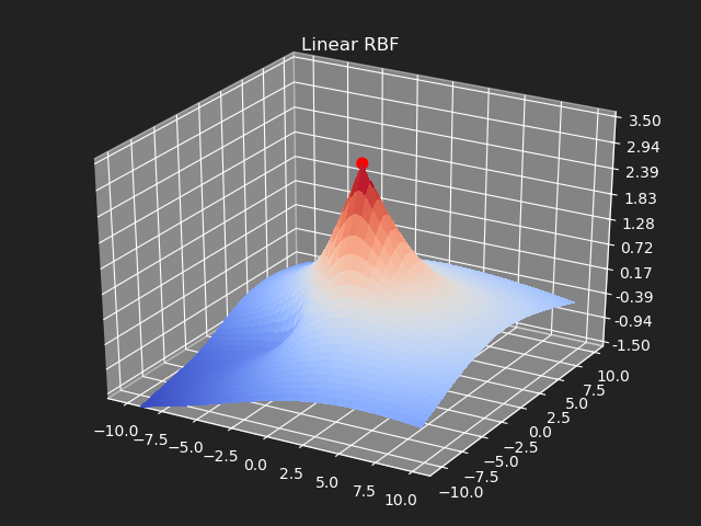
Using the distance value by itself is called a linear radial basis function or linear RBF. Any function that we apply to the distance values is called a radial basis function and can be used to change the interpolation between data points.
Example RBF Kernels
Given a set of input data points and associated output values, plot the results with various RBFs.
$$ M = \begin{bmatrix} 0.0 & 0.0 \\ 2.0 & 3.0 \\ 3.0 & -1.0 \\ -4.0 & -2.0 \\ -2.0 & 3.0 \end{bmatrix} B = \begin{bmatrix} 3.0 \\ 0.5 \\ 1.0 \\ -1.0 \\ 1.0 \end{bmatrix} $$
Linear
Using the distance values directly.
Gaussian
For RBF kernels other than linear, we introduce a radius or falloff parameter. In order to get consistant results, we want the distances to be in the same range of values so the falloff remains consistant no matter how many input features we are providing. To do this, we just normalize the distance matrix before applying the RBF function. Note we use the same distance norm on both the feature matrix and the input vector
// Eigen
double distanceNorm = m.norm();
m /= distanceNorm;
inputDistance /= distanceNorm;
# numpy
distance_norm = np.linalg.norm(M)
M /= distance_norm
input_distance /= distance_norm
The gaussian kernel is a common bell-curve function to smooth the interpolation between samples. Note however when the input goes outside of the sample value range, the results can be undesirable.
// Eigen
struct Gaussian {
  Gaussian(const double& radius) {
    static const double kFalloff = 0.707;
    r = radius > 0.0 ? radius : 0.001;
    r *= kFalloff;
  }
  const double operator()(const double& x) const { return exp(-(x * x) / (2.0 * r * r)); }
  double r;
};

m = m.unaryExpr(Gaussian(radius));
# numpy
def gaussian(matrix, radius):
    radius *= 0.707
    result = np.exp(-(matrix * matrix) / (2.0 * radius * radius))
    return result

M = gaussian(M, radius=radius)
Thin-Plate
// Eigen
struct ThinPlate {
  ThinPlate(const double& radius) { r = radius > 0.0 ? radius : 0.001; }
  const double operator()(const double& x) const {
    double v = x / r;
    return v > 0.0 ? v * v * log(v) : v;
  }
  double r;
};

m = m.unaryExpr(ThinPlate(radius));
# numpy
def thin_plate(matrix, radius):
    v = matrix / radius
    v = np.where(v > 0, v * v * np.log(v), v)
    return v

M = thin_plate(M, radius=radius)
Multi-Quadratic Biharmonic
// Eigen
struct MultiQuadraticBiharmonic {
  MultiQuadraticBiharmonic(const double& radius) : r(radius) {}
  const double operator()(const double& x) const { return sqrt((x * x) + (r * r)); }
  double r;
};

m = m.unaryExpr(MultiQuadraticBiharmonic(radius));
# numpy
def multi_quadratic_biharmonic(matrix, radius):
    result = np.sqrt((matrix * matrix) + (radius * radius))
    return result

M = multi_quadratic_biharmonic(M, radius=radius)
Inverse Multi-Quadratic Biharmonic
// Eigen
struct InverseMultiQuadraticBiharmonic {
  InverseMultiQuadraticBiharmonic(const double& radius) : r(radius) {}
  const double operator()(const double& x) const { return 1.0 / sqrt((x * x) + (r * r)); }
  double r;
};

m = m.unaryExpr(InverseMultiQuadraticBiharmonic(radius));
# numpy
def inv_multi_quadratic_biharmonic(matrix, radius):
    result = 1.0 / np.sqrt((matrix * matrix) + (radius * radius))
    return result

M = inv_multi_quadratic_biharmonic(M, radius=radius)
Beckert Wendland C2 Basis
// Eigen
struct BeckertWendlandC2Basis {
  BeckertWendlandC2Basis(const double& radius) { r = radius > 0.0 ? radius : 0.001; }
  const double operator()(const double& x) const {
    double v = x / r;
    double first = (1.0 - v > 0.0) ? pow(1.0 - v, 4) : 0.0;
    double second = 4.0 * v + 1.0;
    return first * second;
  }
  double r;
};

m = m.unaryExpr(BeckertWendlandC2Basis(radius));
# numpy
def beckert_wendland_c2_basis(matrix, radius):
    arg = matrix / radius
    first = np.zeros(matrix.shape)
    first = np.where(1 - arg > 0, np.power(1 - arg, 4), first)
    second = (4 * arg) + 1
    result = first * second
    return result

M = beckert_wendland_c2_basis(M, radius=radius)
Regularization
So far we have not used the regularization parameter described earlier. Regularization is useful if there are many samples and we want the resulting generalized interpolation to be smooth and we don’t care as much for the result to exactly hit the input data points. This probably won’t be used much in cases where artists are manually entering in samples such as in a corrective shape or set driven key situations. But if the sample data is from a large generated data set, regularization can be used to create a smoother generalized interpolation of that data set.
Conclusion
Finishing up this post, you should have a good intuition of what RBF is and how to apply it. You can view a C++ node implementation of all of this on my Github. Some thing to keep in mind is that it is usually not a good idea to use more than one euler rotation as inputs into the system. Euler rotations can lead to undesirable results due to gimbal lock and the fact there can be multiple values to represent the same rotation. In a future post, I will go over how to use the quaternion rotation as a more reliable input in to the RBF system.